Variational Inference
RECAP: Approximate Bayesian Method
Bayesian inference can be summarized as follows:
- Using a model for the data distribution (likelihood, $L(\theta\mid X)$) and the prior distribution ($\pi(\theta)$) of the parameter,
- derive the posterior probability ($\pi(\theta\mid X)$), and
- perform inference regarding the parameters based on the posterior distribution.
However, when the likelihood is complex or the dataset is very large, calculating the posterior probability becomes challenging.
As a result, various approximate Bayesian methods have been proposed.
Variational Inference
Variational inference is a type of approximate Bayesian method. It involves finding a distribution that is close to the posterior distribution while being relatively easier to sample from, and using it for inference. Typically, a class of candidate distributions for the posterior is predefined, and the optimal distribution is selected from this class.
Variational inference is generally faster than MCMC.
Even outside the Bayesian method, MCMC is used as a method for sampling from distributions, while variational inference is used as a technique for approximating distributions.
To explain the process of variation inference, consider the following assumptions:
- Data: $\mathbf{X} = (X_1, \cdots, X_n)$
- Hidden variables (latent variables): $\mathbf{Z} = (Z_1, \cdots, Z_m)$
- Additional parameter: $\alpha$
- Objective: Find a tractable approximate distribution $q(\mathbf{Z} \mid \nu)$ that is close to the posterior distribution $p(\mathbf{Z} \mid \mathbf{X}, \alpha)$, in order to generate samples $\mathbf{Z}$ or approximate posterior statistics.
Finding the Approximate Distribution
First, let’s find $q(\mathbf{Z} \mid \nu)$ that is close to $p(\mathbf{Z} \mid \mathbf{X}, \alpha)$. This can be viewed as the problem of identifying $\nu$ such that $q(\mathbf{Z} \mid \nu)$ becomes as close as possible to $p(\mathbf{Z} \mid \mathbf{X}, \alpha)$.
Here, $\nu$ is referred to as the variational parameter.
Now, how do we define the criterion for the “closeness” between these two distributions? While there are various possible criteria, the most widely used is the Kullback–Leibler (KL) divergence.
KL Divergence
KL divergence is a concept derived from information theory, used to measure the closeness between two distributions.
\[\begin{aligned} KL(q \parallel p) &= E_q \left( \log \frac{q(\mathbf{Z})}{p(\mathbf{Z} \mid \mathbf{X})} \right)\\ &= E_q (\log q(\mathbf{Z}) - \log p(\mathbf{Z} \mid \mathbf{X}))\\ &= \sum_{\mathbf{z}} \log \left( \frac{q(\mathbf{z})}{p(\mathbf{z} \mid \mathbf{X})} \right) q(\mathbf{z}) \quad (\text{discrete})\\ &= \int \log \left( \frac{q(\mathbf{z})}{p(\mathbf{z} \mid \mathbf{X})} \right) q(\mathbf{z}) d\mathbf{z} \quad (\text{continuous}) \end{aligned}\]- If $q(\mathbf{Z}) = p(\mathbf{Z} \mid \mathbf{X})$, then $KL(q \parallel p) = 0$.
- $KL(q \parallel p) \geq 0$
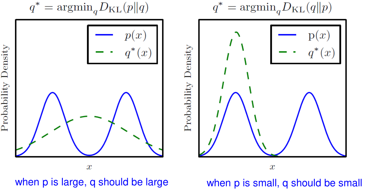
- Asymmetric: $KL(q \parallel p) \neq KL(p \parallel q)$
KL divergence cannot be a distance because of its asymmetricity.
Minimize KL Divergence
Again, let’s return to the original problem. Using the KL divergence, the problem can be expressed as:
\[q^\ast = \arg\min_{q\in Q} KL\left(q(\mathbf{Z}) \parallel p(\mathbf{Z} \mid \mathbf{X})\right).\]Directly calculating the KL divergence requires the logarithm of the unknown distribution $p$, which is not feasible in practice. Instead, a commonly used substitute is the evidence lower bound (ELBO).
Evidence Lower Bound (ELBO)
\[\begin{aligned} KL(q(\mathbf{Z}) \parallel p(\mathbf{Z} \mid \mathbf{X})) &= E_q \left( \log \frac{q(\mathbf{Z})}{p(\mathbf{Z} \mid \mathbf{X})} \right)\\ &= E_q (\log q(\mathbf{Z})) - E_q (\log p(\mathbf{Z} \mid \mathbf{X}))\\ &= E_q (\log q(\mathbf{Z})) - E_q (\log p(\mathbf{Z}, \mathbf{X})) + E_q (\log p(\mathbf{X}))\\ &= E_q (\log q(\mathbf{Z})) - E_q (\log p(\mathbf{Z}, \mathbf{X})) + \log p(\mathbf{X})\\ &= -ELBO(q) + \log p(\mathbf{X}) \end{aligned}\]Thus, ELBO is defined as follows:
\[ELBO(q) = E_q\left(\log p(\mathbf{Z}, \mathbf{X})\right) - E_q\left(\log q(\mathbf{Z})\right).\]In this case, since $\log p(\mathbf{X})$ is constant with respect to $q$, it is not needed in the KL divergence minimization problem.
Therefore, the problem can be written as follows:
\[\begin{aligned} q^\ast &= \arg\min_{q\in Q} KL\left(q(\mathbf{Z}) \parallel p(\mathbf{Z} \mid \mathbf{X})\right)\\ &= \arg\max_{q\in Q} ELBO\left(q(\mathbf{Z})\right) \end{aligned}\]$\log p(X)$ is the likelihood of the observed data, alse called the evidence, and ELBO refers to the lower bound of this evidence.
ELBO can be written as follows.
\[\begin{aligned} ELBO(q) &= E_q \left( \log p(\mathbf{Z}, \mathbf{X}) \right) - E_q (\log q(\mathbf{Z}))\\ &= E_q \left( \log p(\mathbf{X} \mid \mathbf{Z}) \right) + E_q (\log p(\mathbf{Z})) - E_q (\log q(\mathbf{Z}))\\ &= E_q \left( \log p(\mathbf{X} \mid \mathbf{Z}) \right) - E_q \left( \log \frac{q(\mathbf{Z})}{p(\mathbf{Z})} \right)\\ &= E_q \left( \log p(\mathbf{X} \mid \mathbf{Z}) \right) - KL \left( q(\mathbf{Z}) \parallel p(\mathbf{Z}) \right) \end{aligned}\]In the last expression, $\log p(\mathbf{X} \mid \mathbf{Z})$ in the first term represents the probability of the observed data $\mathbf{X}$ (in log scale) given the latent variables $\mathbf{Z}$, which can be seen as the log-likelihood of $\mathbf{Z}$. Therefore, the first term becomes the expectation of log-likelihood of $\mathbf{Z}$. Maximizing the ELBO is equivalent to increasing $p(\mathbf{X} \mid \mathbf{Z})$, or finding a $q(\mathbf{Z})$ that better explains the data.
The second term in the last expression is the KL divergence between the prior distribution of $\mathbf{Z}$, $p(\mathbf{Z})$, and $q(\mathbf{Z})$. Maximizing ELBO is therefore also about finding a $q(\mathbf{Z})$ that is close to the prior distribution $p(\mathbf{Z})$.
In other words, maximizing ELBO($q$) means finding an appropriate $q$ that balances the likelihood and the prior.
Variational Family
\[\begin{aligned} q^\ast &= \arg\min_{q\in Q} KL\left(q(\mathbf{Z}) \parallel p(\mathbf{Z} \mid \mathbf{X})\right)\\ &= \arg\max_{q\in Q} ELBO\left(q(\mathbf{Z})\right) \end{aligned}\]In the above problem, the task of finding $q$ depends on the choice of the family of distributions $Q$, which affects the computational complexity. A commonly used assumption is the mean-field variational family, which refers to a set of distributions where the latent variables are independent and each depends on a separate variational factor. That is, $q(\mathbf{Z}) = \prod_{j=1}^m q_j(Z_j)$. Therefore, the problem becomes finding the set of \(\{ q_j^\ast \}\) that maximizes ELBO($q$).
This variational family does not depend on $\mathbf{X}$.
While more complex families can be considered, they generally increase the computational complexity. The specific choice of the family depends on the problem, and once the family is defined, an appropriate optimization algorithm should be applied.
Given the $\mathbf{X}$ and the variational family $Q$, once the set \(\{ q_j^\ast \}\) is found, it can be used to generate $Z_i$ as needed. The generated \(\{Z_i\}\) can also be used to create data $\mathbf{X^\ast}$ that is similar to the original $\mathbf{X}$ (generative model).