Unconstrained Optimization

Theory of Unconstrained Optimization

Optimality Conditions

Lemma:

Suppose that $f: \mathbb{R}^n \rightarrow \mathbb{R}$ is differentiable at $\bar{x}$. If there is a vector $d \in \mathbb{R}$ such that $\nabla f(\bar{x})^Td < 0$, then $d$ is a descent direction of $f$ at $\bar{x}$.

• sketch of proof: $f(x+\lambda d) \approxeq f(x) + \lambda \nabla f(x)^Td \le f(x)$ for $\lambda \ge 0$.

This is the basic principle of gradient descent or SGD.

Theorem: First-Order Necessary Optimality Conditions (FONC)

Suppose $f: \mathbb{R}^n \rightarrow \mathbb{R}$ is differentiable at \(x^*\). If \(x^*\) is a local minimum, then \(\nabla f(x^*) = 0\).

Theorem: Second-Order Optimality Conditions

Suppose $f: \mathbb{R}^n \rightarrow \mathbb{R}$ is twice differentiable at \(x^*\).
[Necessary] If \(x^*\) is a local minimum, then \(\nabla f(x^*) = 0\) and \(\nabla^2 f(x^*)\) is positive semidefinite.
[Sufficient] If \(\nabla f(x^*) = 0\) and \(\nabla^2 f(x^*)\) is positive definite, then $x^*$ is a strict local minimum.

It is easy to understand by substituting $y=f(x)$.

Determining Local Optima

1. Find the critical points of $f(x,y)$ by solving the system of simultneous equations: $f_x=0, f_y=0$.

2. Let $D(x,y)=f_{xx}f_{yy} - f_{xy}^2$.

3. Then

   1. $D(a,b)>0$ and $f_{xx}(a,b)<0$ implies that $f(x,y)$ has a local maximum at the point $(a,b)$.

   2. $D(a,b)>0$ and $f_{xx}(a,b)>0$ implies that $f(x,y)$ has a local minimum at the point $(a,b)$.

   3. $D(a,b)<0$ implies that $f(x,y)$ has neither a local maximum nor a local minimum at the point $(a,b)$, it has instead a saddle point.

   4. $D(a,b)=0$ implies that the test is inconclusive, so some other technique must be used to solve the problem.

Line Search Strategy

Line Search

Line search is a technique in numerical analysis used to find (approximate) solutions and can be appropriately applied to complex differentiable functions.

In principle, starting from a given point $x_k$, a search direction $p_k$ is computed, and then a new point $x_{k+1}$ is found by moving in that direction by a positive scalar step length $\alpha_k$:

\[x_{k+1} = x_k + \alpha_k p_k.\]

Thus, the line search method is concerned with selecting an appropriate search direction and step length.

The step length is analogous to the learning rate in typical learning algorithms.

$p_k$ is chosen as a descent direction, i.e. $p_k^T\nabla f_k <0$, and in many line search methods, $p_k$ takes the following form:

\[p_k = -B_k^{-1}\nabla f_k\]

where $B_k$ is a symmetric and nonsingular matrix.

The Wolfe Conditions

The Wolfe condition provide criteria for determining the step length in an inexact line search method.

• [Armijo condition : $f(x_k + \alpha_k d_k) \leq f(x_k) + c_1 \alpha_k \nabla f(x_k)^T d_k$]
  The function value at the new point must decrease sufficiently compared to the current point.
• [Curvature condition : $\nabla f(x_k + \alpha_k d_k)^T d_k \geq c_2 \nabla f(x_k)^T d_k$]
  The gradient at the new point must be at least $c_2$ times the original gradient. (This ensures the step does not go too far or end up in a very flat region.)

Line Search Methods

• Steepest Descent
  • $x_{k+1} = x_k - \alpha_k \nabla f_k$
  • The rate-of-convergence is linear.
  • Global convergence if $\alpha_k$ satisfies the Wolfe conditions.

This is what we commonly refer to as the gradient descent method.

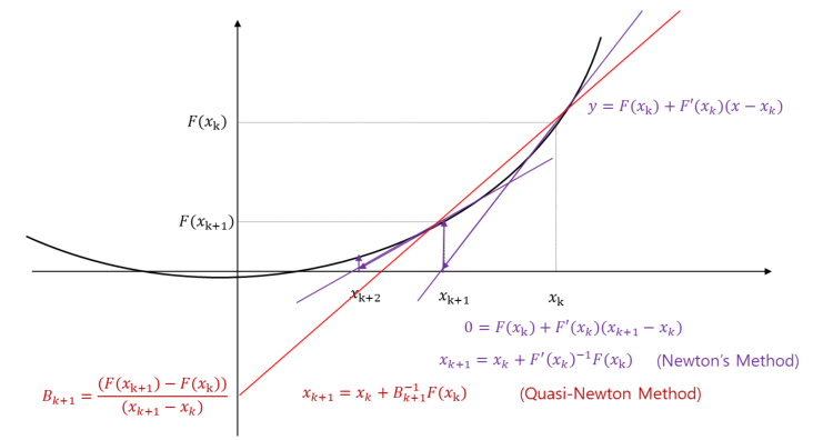
• Quasi-Newton Method
  • $x_{k+1} = x_k - \alpha_k B_k^{-1}\nabla f_k$
  • The rate-of-convergence is superlinear.
  • Global convergence if $\alpha_k$ satisfies the Wolfe conditions.
  • The BFGS method is the most popular.
• Newton’s Method
  • $x_{k+1} = x_k - (\nabla^2 f_k)^{-1}\nabla f_k$
  • The rate-of-convergence is quadrtic.
  • Local convergence.