Projective Geometry and Homography
최근 CV 연구 분야에서는 3D에 대한 관심이 높아지고 있다. 여기서는 3D image 연구의 기본 개념에 대해서 다뤄보고자 한다.
Projective Geometry
우리가 일반적으로 알고있는 기하학은 Euclidean geometry $\mathbb{R}^N$라고 한다. Projective geometry $\mathbb{P}^N$는 간단하게 Euclidean + infinity points라고 말할 수 있다.
가장 특징적인 차이는, projective geometry에서는 Euclidean과 다르게 평행한 두 직선이 어떤 한 점에서 만난다는 것이다.
이러한 projective geometry를 수학적으로 표현하는 방법이 homogeneous coordinate이다. (Euclidean geometry의 coordinate은 inhomogeneous coordinate이라고 말한다.)
Homogeneouse Coordinate
아래 그림의 점을 inhomogeneous coordinate로 다음과 같이 표현한다고 하자.
\[\mathbf{x} = (x_1, x_2)^T = \begin{bmatrix} x_1 \\ x_2 \end{bmatrix} \in \mathbb{R}^2\]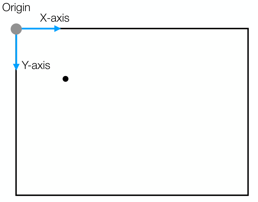
동일한 점을 homogeneous coordinate로 나타내면 다음과 같다.
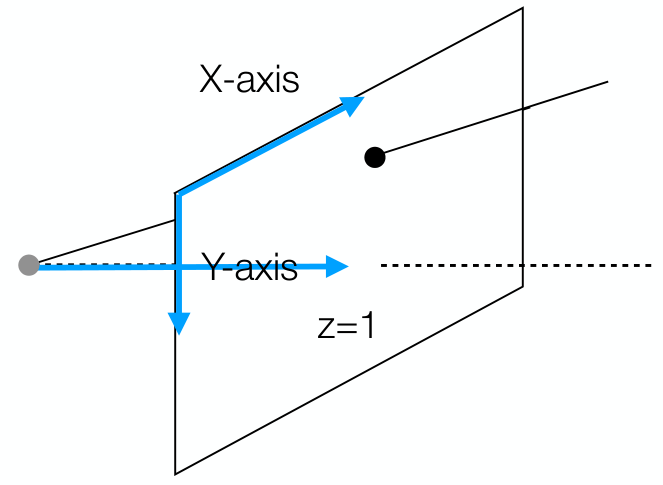
\[\mathbf{x} = (x_1, x_2, 1)^T = \begin{bmatrix} x_1 \\ x_2 \\ 1\end{bmatrix} \in \mathbb{P}^2\]Homogeneous coordinate의 성질 중 하나는 up-to scale로써, 다음 성질이 성립한다. 즉, $\mathbb{P}^2$에서의 DoF는 2가 된다.
\[\begin{bmatrix} x_1 \\ x_2 \\ 1 \end{bmatrix} \equiv \begin{bmatrix} kx_1 \\ kx_2 \\ k \end{bmatrix} \in \mathbb{P}^2\]$\mathbb{R}^2$에서의 point는 $\mathbb{P}^2$에서의 line이 된다.
Homogenous Coordinates in Projective Space $\mathbb{P}^2$
$\mathbb{P}^2$에서 $(0,0,0)$은 정의되어 있지 않다: \(\mathbb{P}^2 = \mathbb{R}^3 - \{(0,0,0)\}\)
$\mathbb{P}^2$에서 $\mathbb{R}^2$로 변환은 다음과 같다: $(x_1, x_2, x_3)^T = (x_1/x_3, x_2/x_3)^T$
Ideal point (point at infinity)는 다음과 같이 정의된다: \(\begin{bmatrix} x_1 \\ x_2 \\ 0 \end{bmatrix}\)
Ideal point가 있으면, 2D image에서 parallel line이 결국 만나게되는 현상을 표현할 수 있다.

Representing 2D Lines in Homogenous Coordinates
일반적으로 line equation은 다음과 같이 표현된다.
\[\{ (x_1, x_2) \mid a x_1 + b x_2 + c = 0 \}\]이를 다시 쓰면,
\[\begin{bmatrix} x_1 & x_2 & 1 \end{bmatrix} \begin{bmatrix} a \\ b \\ c \end{bmatrix} = 0\]Homogenous coordinates에서 $\mathbf{l} = (a,b,c)^T$라고 하면, line $\mathbf{l}$은 다음과 같이 쓸 수 있다.
\[\{ \mathbf{x} \mid \mathbf{x}^T\mathbf{l} = 0 \}\]The Line Joining Two Points
Homogenous coordinates에서 두 점 $\mathbf{x}, \mathbf{x’}$을 모두 지나는 line $\mathbf{l}$은 두 점의 cross product로 구한다.
\[\mathbf{l} = \mathbf{x} \times \mathbf{x'}\]- Proof: $\mathbf{l}^T \mathbf{x} = \mathbf{l}^T \mathbf{x’} = 0$ 으로, $\mathbf{l}$은 $\mathbf{x}, \mathbf{x’}$ 모두에 대해 orthogonal하다. 즉, $\mathbf{l} = \mathbf{x} \times \mathbf{x’}$ 이다.
Intersection of Lines
Homogenous coordinates에서 두 line $\mathbf{l}, \mathbf{l’}$의 intersection $\mathbf{x}$은 두 line의 cross product로 구한다.
\[\mathbf{x} = \mathbf{l} \times \mathbf{l'}\]- Proof: $\mathbf{x}$는 두 line 모두에 대해서 위에 놓여져 있는 점이므로, $\mathbf{l}^T \mathbf{x} = \mathbf{l’}^T \mathbf{x} = 0$.
Parallel Lines and Vanishing Points
두 line $\mathbf{l} = \begin{pmatrix} -1, 0, 1 \end{pmatrix}^T$, $\mathbf{l’} = \begin{pmatrix} -1, 0, 2 \end{pmatrix}^T$을 가정하자. 이는 각각 $-x + 1 = 0$, $-x + 2 = 0$과 일치하므로 parallel line이 된다.
두 line을 지나는 점 $\mathbf{x}$는 다음과 같다.
\[\mathbf{x} = \mathbf{l} \times \mathbf{l'} = \begin{bmatrix} 0 \\ 1 \\ 0 \end{bmatrix}\]$\mathbf{x}$의 마지막 element가 0이므로 ideal point임을 알 수 있다.
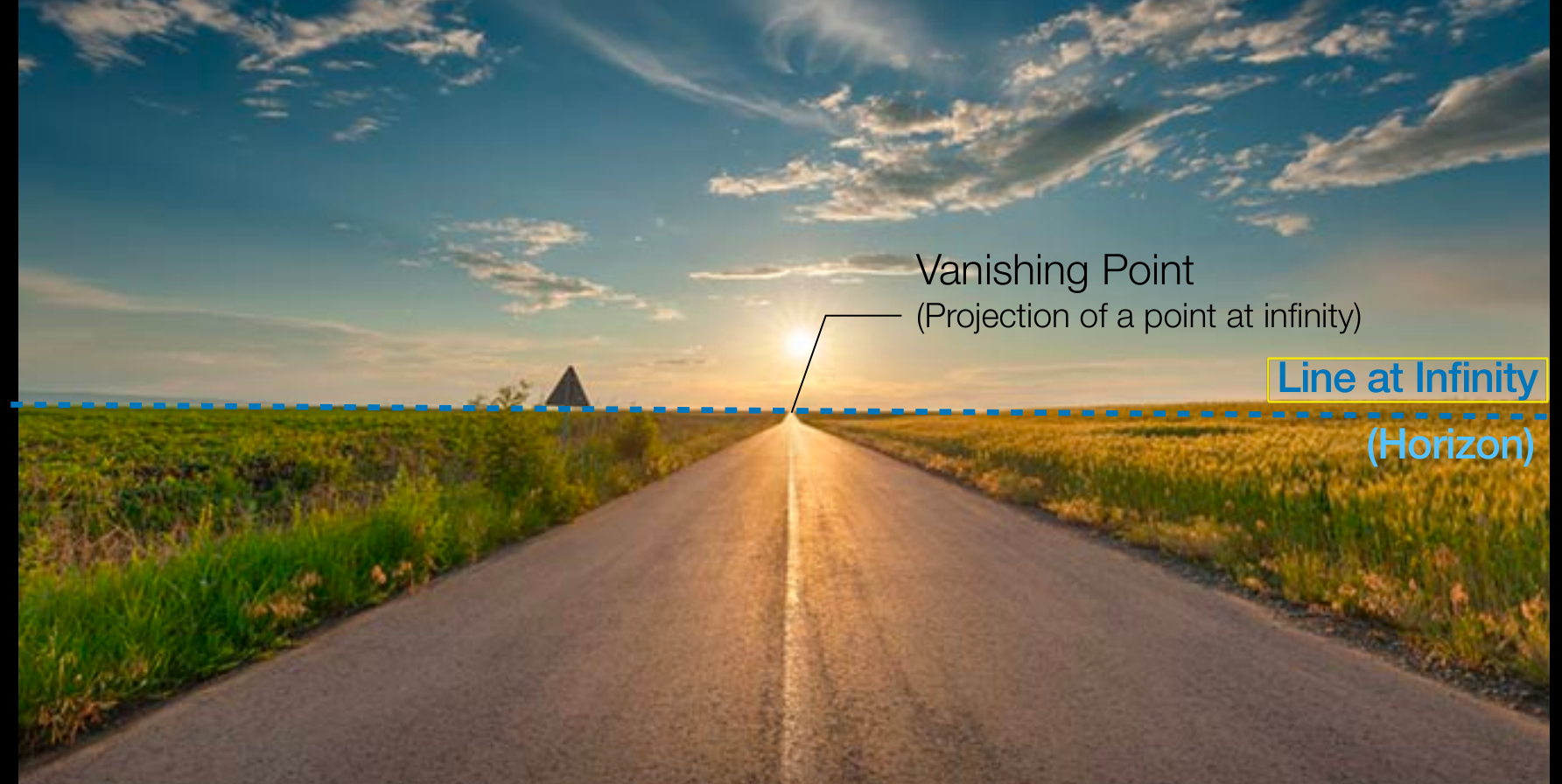
위 예시를 좀 더 일반화 하면, $(-1, 0, c) \cdot (0, 1, 0) = 0$이 되므로, 모든 parallel line $(-1, 0, c)$이 $\mathbf{x}$에서 만나는 것을 알 수 있다. 이러한 ideal point를 vanishing point라고 한다.
Vanishing point는 방향이 같은 경우, 즉 어떤 line을 평행이동 했을 때는 변하지 않지만, 각도가 바뀌는 경우에는 vanishing point가 바뀌게 된다.
Ideal Points and Line at Infinity
앞서 설명했듯이, ideal point는 다음과 같이 표현된다: $(x_1, x_2, 0)^T$.
이 때, 모든 ideal point는 하나의 line에 놓여져 있는데, 이를 line at infinity라고 한다.
\[\mathbf{l}_\infty = (0,0,1)^T\]- Proof: $(x_1, x_2, 0)\cdot(0,0,1) = 0$
Projective Transformation (Homography)
Homography
Homography는 invertible mapping $h: \mathbb{P}^2 \rightarrow \mathbb{P}^2$로써, $\mathbf{x_1}, \mathbf{x_2}, \mathbf{x_3}$이 동일한 line에 존재하면, $h(\mathbf{x_1}), h(\mathbf{x_2}), h(\mathbf{x_3})$ 역시 동일한 line에 존재하는 성질을 갖는다.
Homography는 projectivity, collineation, projective transformation이라고도 불린다.
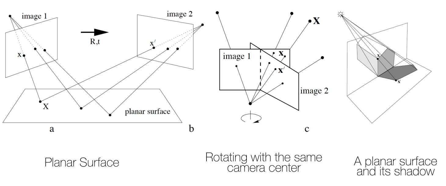
CV에서 homography란 일반적으로 plane-to-plane mapping을 의미한다.
다음은 homography의 예시이다.


Homogenous Matrix
Homography는 3x3 non-singular matrix로 나타낼 수 있다.
\[\mathbf{x'} = \mathbf{Hx}\] \[\begin{bmatrix} x'_1 \\ x'_2 \\ x'_3 \end{bmatrix} = \begin{bmatrix} h_{11} & h_{12} & h_{13} \\ h_{21} & h_{22} & h_{23} \\ h_{31} & h_{32} & h_{33} \end{bmatrix} \begin{bmatrix} x_1 \\ x_2 \\ x_3 \end{bmatrix}\]이 때, H를 homogenous matrix라고 하며, up-to scale 성질을 갖는다 (DoF=8).
Central Projections
특정한 point (center of projection)으로부터 나오는 ray를 따라 한 plane의 점이 다른 plane에 projection되는 경우, 이를 central projection이라고 한다.
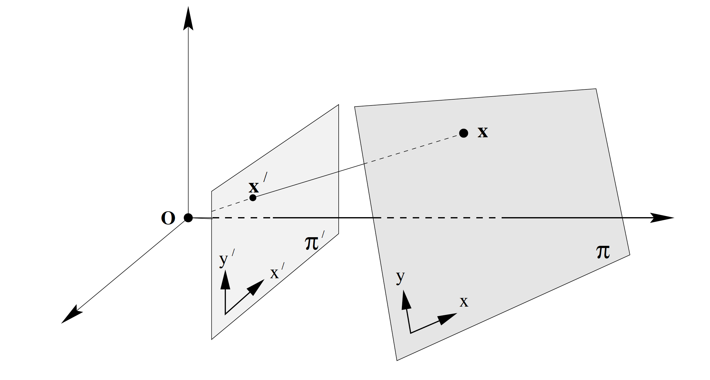
Central projection은 homography mapping으로 표현된다: $\mathbf{x’} = \mathbf{Hx}$
Hierarchy of Transformations
Translation
Transformation $x_i \rightarrow x_i+t_i$을 translation이라고 하며, 다음과 같이 쓸 수 있다. (왼쪽이 inhomogeneous, 오른쪽이 homogeneous coordinate을 나타낸다.)
\[\mathbf{x}' = \mathbf{x} + \mathbf{t} \iff \mathbf{x}' = \begin{bmatrix} \mathbf{I}_{2 \times 2} & \mathbf{t} \\ \mathbf{0}_{1 \times 2} & 1 \end{bmatrix} \mathbf{x}\]Euclidean (Rigid) Transform
Rotation 후 translation을 적용하는 transformation이다.
\[\mathbf{x}' = \mathbf{Rx} + \mathbf{t} \iff \mathbf{x}' = \begin{bmatrix} \mathbf{R} & \mathbf{t} \\ \mathbf{0}_{1 \times 2} & 1 \end{bmatrix} \mathbf{x}\]여기서 R은 special orthogonal group $(R^{-1}=R^T)$에 속하는 matrix로 다음과 같다.
\[\mathbf{R} = \begin{bmatrix} \cos \theta & -\sin \theta \\ \sin \theta & \cos \theta \end{bmatrix}\]CV에서는 rotation과 translation이 동시에 적용되는 경우, rotation을 먼저 적용한 후 translation을 적용하는 것이 일반적이다.
이 외에도 similarity transform, affine transform 등이 있다.
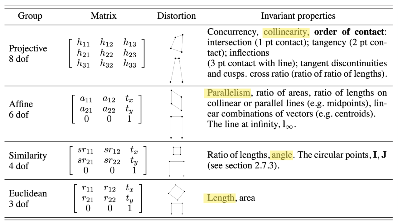
Affine transformation은 parallel line을 mapping한 line 역시 parallel하다는 성질이 있다.
Estimate Homography
Up-to-scale 성질을 고려하면, homography를 다음과 같이 표현할 수 있다.
\[\begin{bmatrix} x'_i \\ y'_i \\ 1 \end{bmatrix} = \begin{bmatrix} h_{11} & h_{12} & h_{13} \\ h_{21} & h_{22} & h_{23} \\ h_{31} & h_{32} & h_{33} \end{bmatrix} \begin{bmatrix} x_i \\ y_i \\ 1 \end{bmatrix}\]이 때, 한 point에 대한 mapping 정보 $(x_i, y_i, 1), (x’_i, y’_i, 1)$가 있다면, 두 개의 linear equation이 나오게 된다.
우리는 8개의 variable에 대한 값을 정해야 하므로, 총 4쌍에 대한 mapping 정보가 있으면 homography의 정보를 모두 구할 수 있다.
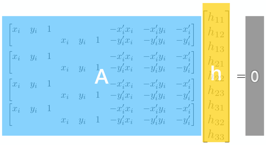
만약, 우리가 더 많은 정보가 있으나, 그 중 일부가 ‘noisy’하여 연립방정식의 solution이 존재하지 않게 되는 경우, 이는 연립방정식의 exact solution을 구하는 것이 아닌 $\Vert \mathbf{Ah}\Vert$를 minimze하는 $\mathbf{h}$를 찾는 optimization 문제가 된다.