Monte-Carlo Method

Monte Carlo Method

The Monte-Carlo method is a technique used to approximate a value (or function value) by utilizing random samples generated from a probability distribution.

This method relies on the law of large number (LLN).

• LLN: Given $X_1, \cdots, X_n \overset{i.i.d.}{\sim} f$,

\[\bar{X}_n = \frac{1}{n} \sum_{i=1}^n X_i \overset{p}{\to} E(X_1).\]

Let the value we wish to compute be denoted as $\theta$, and suppose $\theta$ can be expressed as the expectation of a certain random variable, i.e., $\theta = E(h(X)), X \sim f$.

If $X_1, \cdots, X_n$ are random samples generated from $f$, then by the LLN, the following holds:

\[\frac{1}{n}\sum_{i=1}^n h(X_i) \overset{p}{\to} E(h(X)) = \theta.\]

Thus, the Monte Carlo method requires an algorithm generating random samples from the given probability distribution (random number generation).

Algorithms for generating random samples from most well-known probability distributions have been studied and are readily available in R and Python.

Sampling Methods

Inverse CDF

The inverse CDF sampling method utilizes the probability integral transform (PIT).

• PIT: For a continuous random variable $X$ with a CDF $F_X$, $F_X(X)$ follows $\text{Unif}(0,1)$.

If $F_X(X) \sim U$ and $U$ is distributed as $(\text{Unif}(0,1))$, the the following holds:

\[X \sim F_X^{-1}(U) = \inf \{x : F(x) \ge U\}.\]

In other words, if $U_1, \cdots, U_k$ are generated from $(\text{Unif}(0,1))$, then $X_1 = F^{-1}(U_1), \cdots, X_k = F^{-1}(U_k)$ are random samples following $F(x)$.

If it is challenging to obtain $F^{-1}(u)$ directly, the following approach can be used:

1. Identify a suitable sequence $x_1, \cdots, x_m$ within the support of $f(x)$, and compute $u_i = F(x_i)$.
   • The support of $f(x)$ is defined as \(\{x \mid f(x) > 0 \}\).

2. Generated a random variable $U \sim \text{Unif}(0,1)$ and find the closet $u_i \leq U \leq u_j$. Using these, compute $X$ as follows:

   \[X = \frac{u_j - U}{u_j - u_i} x_i + \frac{U - u_i}{u_j - u_i} x_j.\]
   • The value of $X$ a linear interpolation between $(x_i, F(x_i))$ and $(x_j, F(x_j))$.

Example of Inverse CDF

Suppose we aim to randomly generate a variable following the PDF:

\[f(x) = \frac{1}{2} x, 0 < x < 2.\]

The CDF is given by

\[F(x) = \int_{0}^{x} f(y) dy = \frac{1}{4} x^2, 0 < x < 2.\]

The inverse of the CDF is:

\[F^{-1}(u) = \sqrt{4u} = 2 \sqrt{u}, 0 < u < 1.\]

Thus, if $U_1, \cdots, U_k \sim \text{Unif}(0,1)$, then the samples $X_1 = 2 \sqrt{U_1}, \cdots, X_k = 2 \sqrt{U_k}$ are random samples generated from the given $f(x)$.

Rejection Sampling

To generate $X \sim f$, rejection sampling proceeds as follows:

1. Identify a probability distribution $g$ that is easy to sample from and satisfies:

   \[\beta f(x) \leq g(x), 0 < \beta < 1.\]
   • The function $g(x)/\beta = e(x)$ is called the upper envelop of $f(x)$.

   

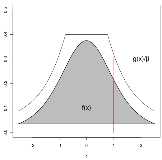
2. Generate a sample $X$ from $g(x)$.

3. Generate $U \sim \text{Unif}(0, 1)$.

4. Accept $X$ as a sample from $f$ if $Ug(X) \leq \beta f(X)$ (equivalently $U \leq f(X)/e(X)$). Otherwise, reject $X$ and return to step 2.

5. Repeat until the desired number of samples is obtained.

Example of Rejection Sampling

Consider the same PDF as the above: $f(x) = \frac{1}{2}x, 0 < x < 2$.

Choose $g(x) = \frac{1}{2}, 0 < x < 2$, which is the PDF of $\text{Unif}(0,2)$. This satisfies $f(x) \leq g(x)/\beta$ with $\beta = 1/2$. The envelope function becomes $e(x) = 2g(x) = 1$.

The rejection sampling algorithm for this case is as follows:

1. Generate $X \sim \text{Unif}(0,2)$.

2. Generate $U \sim \text{Unif}(0, 1)$.

3. Accept $X$ as a sample from $f(x)$ if $U \leq f(X)/e(X) = \frac{1}{2}X$. Otherwise, reject $X$ and repeat.

Importance Sampling

Let’s return to the problem of estimating $\theta = E(h(X))$, where $X \sim f$.

If there exists a distribution $g$ that is easier to sample from and whose support includes the support of $f$, then $\theta$ can be expressed using $g$ as follows:

\[\begin{aligned} \theta &= E_{f}(h(X)) = \int h(x) f(x) dx \\ &= \int h(x) \frac{f(x)}{g(x)} g(x) dx = E_{g} \left( h(X) \frac{f(X)}{g(X)} \right). \end{aligned}\]

Let $X_{1}, \ldots, X_{n}$ be random samples generated from $g$. Define $w^\ast(x) = \frac{f(x)}{g(x)}$. Then, $\theta$ can be approximated as:

\[\hat{\theta} = \frac{1}{n} \sum_{i} h(X_{i}) w^\ast(X_{i}).\]

The function $g$ is referred to as the importance sampling function.

Example of Importance Sampling

Consider the same PDF as the above: $f(x) = \frac{1}{2}x, 0 < x < 2$.

We aim to estimate $\theta = E(X^{2})$.

Since $f(x) = \frac{1}{2}x$ and $0 < x < 2$, the exact value of $E(X^{2})=2$. However, it can also be approximated using importance sampling.

Choose $g(x) = \frac{1}{2}$. Then:

\[\begin{aligned} \theta &= E_{f}(X^{2}) = \int x^{2} f(x) dx \\ &= \int x^{2} (\frac{f(x)}{g(x)}) g(x) dx \\ &= \int x^{2} \cdot x \cdot (\frac{1}{2}) dx \\ &= E_{g}(X^{3}). \end{aligned}\]

Generated $X_{1}, \cdots, X_{n} \sim \text{Unif}(0, 2)$. Then approximate $\theta$ using:

\[\hat{\theta} = \frac{1}{n} \sum h(X_{i}) w^{*}(X_{i}) = \frac{1}{n} \sum X_{i}^{3}.\]