Momentum

Pathological Curvatures

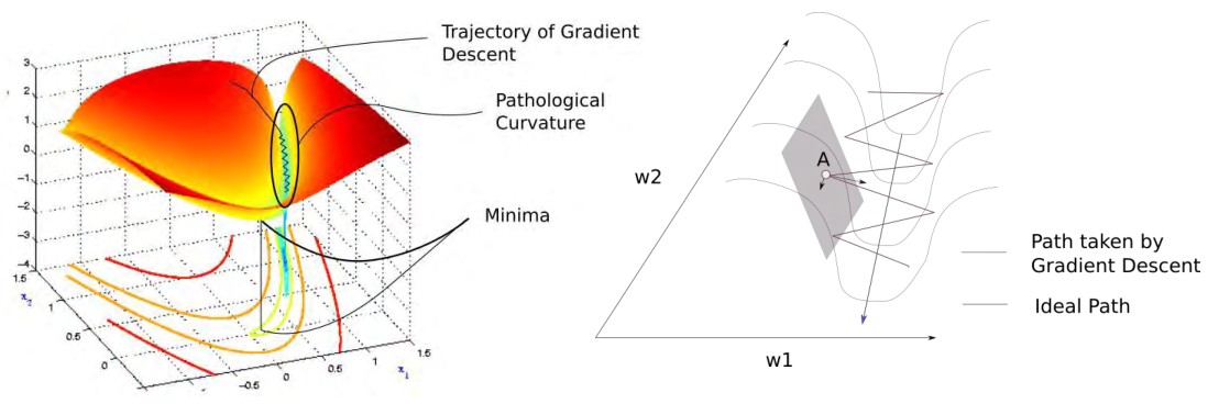
In the above figure, finding the minimum of the loss surface inevitably requires passing through steep valleys. At point $A$, calculating the gradient reveals that the magnitude of the gradient in the $w_1$ direction is much larger than that in the $w_2$ direction. As a result, the next point moves toward the $w_1$ direction rather than the $w_2$ direction where the actual minimum is located.

This zigzagging gradient update behavior is called gradient oscillation.

Momentum

To prevent gradient oscillation, algorithms that maintain the momentum of previous parameters (typically the gradient value from the preceding epoch) are commonly employed.

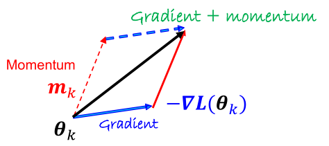
Basic Momentum Algorithm

The momentum algorithm fundamentally refers to maintaining the momentum of the gradient value from the previous epoch through exponential averaging.

• $m_t$: momentum at the $t$-th iteration
• $\beta$: momentum hyperparameter (typically 0.9)
• $\theta_t$: parameter vector at the $t$-th iteration
• $\alpha$: learning rate

\[m_t = \beta m_{t-1} + (1 - \beta) \frac{1}{|B_j|} \sum_{i \in B_j} \nabla_{\theta} \mathcal{L}_i(\theta_{t-1})\] \[\theta_t = \theta_{t-1} - \alpha m_t\]

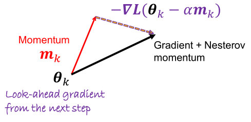
Nesterov Accelerated Gradient (NAG)

NAG calculates the gradient at the future position predicted using momentum and applies it to the current parameter update. This approach leads to faster and more stable convergence.

\[m_t = \beta m_{t-1} + (1 - \beta) \frac{1}{|B_j|} \sum_{i \in B_j} \nabla_{\theta} \mathcal{L}_i(\theta_{t-1} - \alpha m_{t-1})\] \[\theta_t = \theta_{t-1} - \alpha m_t\]

Normalizing Gradients

Gradient descent algorithms adjust parameters based on the magnitude of the gradient. In cases where the loss surface has pathological curvatures, as previous discussed, gradients may vary significantly across different directions, making it difficult to select a stable learning rate for all directions.

To address this issue, gradient normalization techniques are sometimes applied. Using normalized gradients ensures more uniform movement in each direction. However, if the optimization does not precisely reach the minimum, it may oscillate near the minimum without converging.

Subsequent methods such as Adagrad, RMSProp, AdaDelta, and Adam all incorporate gradient normalization techniques.

Adagrad

Adagrad adapts the learning rate for each parameter based on the historical gradient updates. Parameters that have experienced large changes (with large gradients) are updated with a smaller learning rate, as they are likely closer to the optimum. Conversely, parameters with smaller gradient changes receives a larger learning rate to reduce errors more quickly.

This method works well for sparse datasets but has the drawback of a rapidly decaying learning rate, which may cause the learning process to halt prematurely.

\[g_t = \frac{1}{|B_j|} \sum_{i \in B_j} \nabla_{\theta} \mathcal{L}_i(\theta_t)\] \[G_t = G_{t-1} + g_{t-1} \odot g_{t-1}\] \[\theta_t = \theta_{t-1} - \frac{\alpha}{\sqrt{G_t + \epsilon}} g_{t-1}\]

• $G_t$: the cumulative sum of the squared gradients from past iterations
• $\epsilon$: a small constant to prevent division by zero

To avoid increased computation costs, the gradient is calculated only once per update.

RMSProp

RMSProp addresses the rapid decay of the learning rate in Adagrad by using exponential averaging with a parameter $\gamma$ to adjust the influence of past gradients.

\[g_t = \frac{1}{|B_j|} \sum_{i \in B_j} \nabla_{\theta} \mathcal{L}_i(\theta_t)\] \[G_t = \gamma G_{t-1} + (1-\gamma) g_{t-1} \odot g_{t-1}\] \[\theta_t = \theta_{t-1} - \frac{\alpha}{\sqrt{G_t + \epsilon}} g_{t-1}\]

AdaDelta

AdaDelta removes the learning rate parameter and instead uses a parameter $s_t$ related to the change in parameter vector ($\Delta \theta_t$).

\[g_t = \frac{1}{|B_j|} \sum_{i \in B_j} \nabla_{\theta} \mathcal{L}_i(\theta_t)\] \[G_t = \gamma G_{t-1} + (1-\gamma) g_{t-1} \odot g_{t-1}\] \[\Delta \theta_t = - \frac{\sqrt{s_{t-1} + \epsilon}}{\sqrt{G_t + \epsilon}} g_{t-1}\] \[s_t = \gamma s_{t-1} + (1-\gamma) \Delta \theta_t \odot \Delta \theta_t\] \[\theta_t = \theta_{t-1} + \Delta \theta_t\]

Adam

Adam is one of the most widely used algorithms, combining the momentum algorithm and RMSProp. It uses the momentum ($m_t$) and the second moment information of the gradient ($G_t$) to perform parameter updates.

\[g_t = \frac{1}{|B_j|} \sum_{i \in B_j} \nabla_{\theta} \mathcal{L}_i(\theta_t)\] \[m_t = \beta m_{t-1} + (1-\beta) g_{t-1}\] \[G_t = \gamma G_{t-1} + (1-\gamma) g_{t-1} \odot g_{t-1}\] \[\hat{m}_t = \frac{m_t}{1 - \beta^t}, \quad \hat{G}_t = \frac{G_t}{1 - \gamma^t}\] \[\theta_t = \theta_{t-1} - \alpha \frac{\hat{m}_t}{\sqrt{\hat{G}_t + \epsilon}}\]

Recommended hyperparameters: $\beta=0.9$, $\gamma=0.999$, $\epsilon=10^{-8}$.

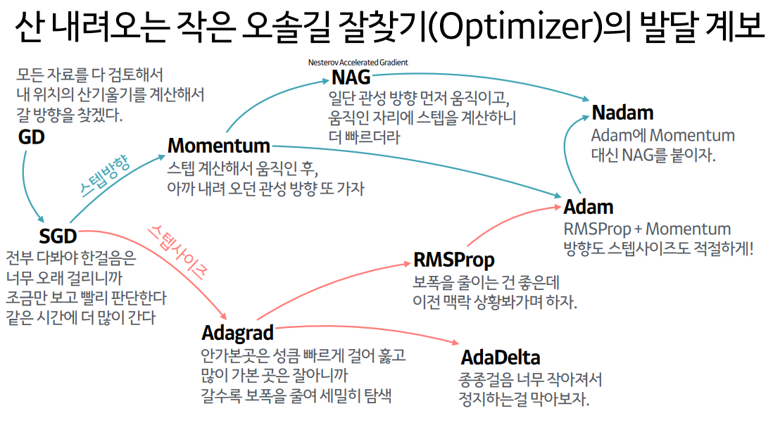
Summary

Here is a helpful diagram summarizing the key points above.