Linear Regression
Linear regression은 가장 간단한 버전의 supervised learning으로, 이는 $Y$가 $X_1, X_2, \dots, X_p$와 linear dependency를 가진다고 가정한다.
현실의 data는 결코 linear가 아니지만, linear model은 구현과 계산이 쉽고, 해석이 가능하다는 큰 장점이 있어 여전히 널리 사용된다.
Simple Linear Regression
Feature 1개에 대한 simple linear regression model은 다음과 같이 쓸 수 있다.
\[Y = \beta_0+\beta_1X+\epsilon\]- $\beta_i$: coefficients, parameters
- $\beta_0$: intercept
- $\beta_1$: slope
- $\epsilon$: error term
위 model의 parameter들의 estimated value와 그를 이용한 prediction은 hat으로 표현한다.
\[\hat{y} = \hat{\beta_0} + \hat{\beta_1}x\]Estimation of Parameters
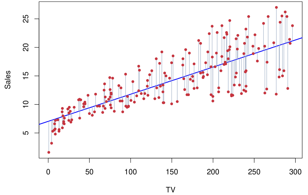
Linear regression model의 parameter에 대한 estimation $\hat{\beta_0}$과 $\hat{\beta_1}$은 아래 Residual Sum of Squares (RSS) 또는 Sum of Squares for Error (SSE)를 minimize하는 값으로 계산한다 (residual: $e_i=y_i-\hat{y_i}$).
\[\text{RSS} = e_1^2+\dots +e_n^2\]Linear regression model에서 residual의 합은 0이 된다.
이러한 방식을 the least sqaures approach라고 하며, 이렇게 구한 $\hat{\beta_1}$과 $\hat{\beta_0}$은 다음과 같다.
\[\hat{\beta}_1 = \frac{\sum_{i=1}^n (x_i - \bar{x})(y_i - \bar{y})}{\sum_{i=1}^n (x_i - \bar{x})^2}, \quad \hat{\beta}_0 = \bar{y} - \hat{\beta}_1 \bar{x}\]여기서 $\bar{y}=\frac{1}{n}\sum_{i=1}^n y_i$, $\bar{x}=\frac{1}{n}\sum_{i=1}^n x_i$ 이다 (sample mean).
$\hat{\beta_1}$은 $X$가 1 unit 증가할 때의 $Y$의 증가량을 나타낸다.
Fraction of Variances
Total Sum of Squares (TSS 또는 SST)는 다음과 같이 정의된다.
\[\text{TSS} = \sum_{i=1}^n(y_i-\bar{y})^2\]Explained Sum of Squares (ESS) 또는 Sum of Squares for Regression (SSR)는 다음과 같이 정의된다.
\[\text{ESS} = \sum_{i=1}^n (\hat{y}_i-\bar{y}_i)^2\]TSS, ESS, 그리고 RSS는 다음과 같은 관계를 갖는다.
\[\text{TSS} = \text{ESS} + \text{RSS}\]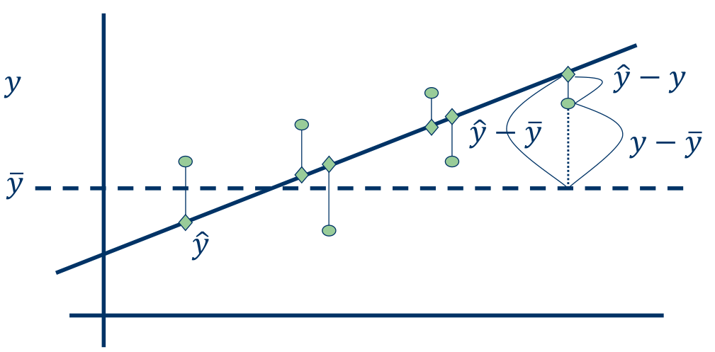
TSS는 전체 data의 variation을 나타내고, ESS는 regression model을 통해 설명된 variation을 나타내며, RSS는 regression model이 설명하지 못하는 variation을 나타낸다. 따라서, RSS가 작을수록 regression model이 data를 잘 설명한다고 볼 수 있다.
$R^2$ (R-squared)
$R^2$는 regression model이 data를 얼마나 잘 설명하는 지를 나타내는 measure이다. 0에서 1사이의 값을 가지며, data의 variance 중 regression model이 설명하는 variance의 비율을 나타낸다.
\[R^2 = \frac{\text{ESS}}{\text{TSS}} = 1-\frac{\text{RSS}}{\text{TSS}}\]$R^2$는 $X$와 $Y$의 correlation coefficient $r=Corr(X,Y)$의 제곱과 같다는 것이 알려져 있다.
$r=Corr(X,Y)$과 $\hat{\beta}$은 다음과 같은 관계를 갖는다.
\[r = \sqrt{\frac{Var(X)}{Var(Y)}}\hat{\beta}_1\]
Standard Error of Estimator
두 estimator들의 standard error는 다음과 같다.
\[SE(\hat{\beta}_1)^2 = \frac{\sigma^2}{\sum_{i=1}^n (x_i - \bar{x})^2}, \quad SE(\hat{\beta}_0)^2 = \sigma^2 \left[\frac{1}{n} + \frac{\bar{x}^2}{\sum_{i=1}^n (x_i - \bar{x})^2}\right],\]여기서 $\sigma^2 = Var(\epsilon)$이다.
이 때, $\sigma$에 대한 estimator로는 Residual Standard Error (RSE)를 사용한다.
\[\text{RSE} = \sqrt{\frac{1}{n - 2} \text{RSS}} = \sqrt{\frac{1}{n - 2} \sum_{i=1}^n (y_i - \hat{y}_i)^2},\]Hypothesis Testing for $\beta_1$
이를 이용하면 X가 Y에 유의미한 영향을 미치는지에 대한 검증이 가능하다.
- $H_0$: X와 Y 사이에는 관계성이 없다. ($\beta_1=0$)
- $H_1$: X와 Y 사이에는 관계성이 있다. ($\beta_1\ne0$)
이는 아래 t-statistic을 활용하며, 계산된 p-value 값을 통해 hypothesis testing을 수행한다.
\[t=\frac{\hat{\beta_1}}{\text{SE}(\hat{\beta_1})}\]이 때, $t$는 $n-2$ degrees of freedom을 갖는 $t$-distribution을 따른다.
Multiple Linear Regression
이제 $p$개의 feature들을 가지는 multiple linear regression model을 생각하자.
\[Y = \beta_0+\beta_1X_1+\dots+\beta_pX_p+\epsilon\]Estimation of Parameters
Multiple linear regression에서도 $\hat{\beta} = (\hat{\beta}_0, \hat{\beta}_1, \dots, \hat{\beta}_p)$는 RSS를 최소화하는 값으로 다음과 같이 표현할 수 있다.
\[\hat{\beta} = (X^TX)^{-1}X^Ty\]이 때, $\beta_j$는 다른 모든 feature의 값들이 고정되어 있을 때, $j$-th feature가 Y에 미치는 평균적인 영향을 의미한다 (partial correlation).
주의: $\beta_j$의 값은 상관관계를 의미하지, 인과관계를 의미하지 않는다!
Multicollinearity
일반적으로 linear regression의 경우 feature들이 서로 independent한 가정 하에서 해석이 이루어지곤 한다. 하지만, 현실의 많은 data는 feature들의 highly correlated된 경우가 많기에 multicollinearity가 나타나는 경우가 많다.
일반적으로 이러한 multicollinearity가 존재하는 경우, correlation이 높은 feature 중 하나만을 사용하는 것이 좋다고 하나, 분석 의도와 설명력을 고려하였을 때 multicollinearity를 포함한 model로 결과를 해석하는 것이 더 합리적일 수 있다.
하지만, multicollinearity가 존재하는 multiple linear regression model에서는 결과를 주의깊게 해석해야만 한다.
다음은 multicollinearity가 존재할 때의 결과 해석에 관한 예시이다.
- $Y$: 월 저축액
| feature | coefficient | std. error | p-value |
|---|---|---|---|
| 월 소득 ($X_1$) | 0.205 | 0.035 | 0.000 |
| feature | coefficient | std. error | p-value |
|---|---|---|---|
| 가구 인원수 ($X_2$) | 1.625 | 1.182 | 0.000 |
| feature | coefficient | std. error | p-value |
|---|---|---|---|
| 월 소득 ($X_1$) | 0.301 | 0.029 | 0.000 |
| 가구 인원수 ($X_2$) | -2.091 | 0.470 | 0.003 |
$X_1$과 $X_2$간에는 positive correlation이 존재하므로, $X_1$과 $X_2$로 만든 linear regression model에는 multicollinearity가 존재한다. 위 결과를 단순히 가구 인원수이 늘어나면 월 저축액이 줄어든다고 해석해서는 안되며, 월 소득이 동일한 경우에 가구 인원수가 적을수록 월 저축액이 늘어난다라고 이해하는 것이 더 올바른 해석이 된다.
Multicollinearity가 존재하는 multiple linear regression model에서는 특정 feature의 parameter의 부호가 바뀌는 경우가 있다. 위 예시의 경우, 이는 $X_2$가 직접적으로 $Y$에 미치는 효과보다 $X_2$가 $X_1$을 통해 간접적으로 $Y$에 미치는 효과가 크기 때문이다.
Multicollinearity이 존재하는 경우, interaction feature를 사용하면 해석이 좀 더 용이하다.
Assumptions of Multiple Linear Regression
- Linearity (선형성)
- Input과 response와의 관계가 linear (가장 중요한 assumption)
- 만족되지 않는 경우, polynomial regression 또는 non-parametric regression 사용
- Homoscedasticity (등분산성)
- Error의 variance가 input에 무관하게 일정
- 만족되지 않는 경우, weighted regression 사용
- Normality (정규성)
- Error가 Gaussian distribution을 따름
- 만족되지 않는 경우, robust regression 사용
Feature Transformation
Categorical Features
Categorical feature들의 경우, 이를 numerical feature로 변경해주는 작업이 필요하다.
만약, gender(여기서는 binary feature로써 생각)를 feature에 포함하는 경우, 이를 아래와 같이 쓸 수 있다.
\[x_i = \begin{cases} 1 & \text{if $i$-th person is female} \\ 0 & \text{if $i$-th person is male} \end{cases}\]Resulting model:
\[y_i = \beta_0 + \beta_1 x_i + \varepsilon_i = \begin{cases} \beta_0 + \beta_1 + \varepsilon_i & \text{if $i$-th person is female} \\ \beta_0 + \varepsilon_i & \text{if $i$-th person is male} \end{cases}\]Ethnicity와 같이 binary하지 않은 feature의 경우에는 다음과 같이 표현한다.
\[x_{i1} = \begin{cases} 1 & \text{if $i$-th person is Asian} \\ 0 & \text{if $i$-th person is not Asian} \end{cases} \\\] \[x_{i2} = \begin{cases} 1 & \text{if $i$-th person is Caucasian} \\ 0 & \text{if $i$-th person is not Caucasian} \end{cases} \\\]Resulting model:
\[y_i = \beta_0 + \beta_1 x_{i1} + \beta_2 x_{i2} + \varepsilon_i = \begin{cases} \beta_0 + \beta_1 + \varepsilon_i & \text{if $i$-th person is Asian} \\ \beta_0 + \beta_2 + \varepsilon_i & \text{if $i$-th person is Caucasian} \\ \beta_0 + \varepsilon_i & \text{if $i$-th person is AA} \end{cases}\]Interaction Features
예를 들어, 아래와 같은 linear model이 있다고 가정하자. 각 feature는 해당 media에 투자하는 광고비를 의미한다. \(\text{sales} = \beta_0 + \beta_1 \times \text{TV} + \beta_2 \times \text{radio} + \epsilon\)
이 때, 우리는 domain knowledge로, radio와 TV에 예산을 나눠서 투자하면, 같은 금액을 한 쪽에만 투자했을 때보다 더 좋은 효과를 거둔다는 것을 알고 있다고 하자.
즉, radio와 TV간 synergy effect가 존재한다. 이 경우, model은 다음과 같이 표현하는게 더욱 정확할 것이다.
\[\begin{aligned} \text{sales} &= \beta_0 + \beta_1 \times \text{TV} + \beta_2 \times \text{radio} + \beta_3 \times \text{(radio}\times\text{TV)} + \epsilon \\ &= \beta_0 + (\beta_1 + \beta_3 \times \text{radio}) \times \text{TV} + \beta_2 \times \text{radio} + \epsilon \end{aligned}\]이러한 interaction term을 추가할 때, p-value 측면에서 interaction term(radio x TV)은 유효하지만, 관련된 original feature 는 유효하지 않다고 판단되는 경우(본 예시에서는 radio)가 있다.
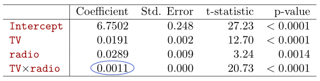
하지만, 이러한 경우에도 original feature를 model에서 제거해서는 안된다!
Interaction term은 main effect가 아닌 interaction effect에 대해서만 영향력을 끼쳐야하는데, original feature가 사라지면 main effect가 interaction term으로 흡수되어 올바른 해석이 어려워진다 (위에서 언급한 multicollinearity를 고려한 해석이 필요).
만약, categorical feature와 numerical feature의 interaction term이 필요한 경우, 아래와 같이 표현할 수 있다.
\[\begin{aligned} \text{balance}_i &\approx \beta_0 + \beta_1 \times \text{income}_i + \begin{cases} \beta_2 + \beta_3 \times \text{income}_i & \text{if student} \\ 0 & \text{if not student} \end{cases} \\ &=\begin{cases} (\beta_0 + \beta_2) + (\beta_1 + \beta_3) \times \text{income}_i & \text{if student} \\ \beta_0 + \beta_1 \times \text{income}_i & \text{if not student} \end{cases} \end{aligned}\]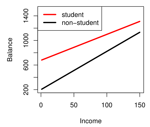
Non-linear Features
Interaction term과 같이, linear model로 표현하기 어려운 feature의 non-linear effect가 존재할 때 다음과 같이 feature의 제곱 등을 포함한 non-linear feature를 추가할 수 있다.
\[\text{mpg} = \beta_0 + \beta_1 \times \text{horsepower} + \beta_2 \times \text{horsepower}^2 + \epsilon\]