Joint Probability Distribution

Joint Probability Distribution

Joint Probability Distribution

A joint probability distribution represents the probabilities of all possible pairs of values that two random variables can take.

1. Discrete joint PMF

   \[p(x,y) = P(X=x, Y=y)\]
   • $0 \leq p(x,y) \leq 1$
   • $\sum_x\sum_y p(x,y) = 1$
   • $P(a<X\leq b, c<Y\leq d) = \sum_{a<x\leq b}\sum_{c<y\leq d}p(x,y)$

2. Continuous joint PDF

   \[P(a < X \leq b, c < Y \leq d) = \int_a^b \int_c^d f(x, y) \, dy \, dx\]
   • $f(x, y) \geq 0$
   • $\int \int f(x, y) \, dx \, dy = 1$
   • $P(a < X \leq b, c < Y \leq d) = \int_c^d \int_a^b f(x, y) \, dx \, dy$

• $E[g(X, Y)] = \int_{-\infty}^{\infty} \int_{-\infty}^{\infty} g(x, y) f(x, y) \, dx \, dy$

• $E[ag(X, Y) + bh(X, Y)] = a E[g(X, Y)] + b E[h(X, Y)]$

Marginal PDF

The marginal PDF is defined as follows:

• $p_X(x) = \sum_y p(x, y)$
• $f_X(x) = \int f(x, y) \, dy$

Two random variables $X$ and $Y$ are independent if the following condition is satisfied:

• Discrete: $p_{X,Y}(x,y) = p_X(x) p_Y(y)$
• Continuous: $f_{X,Y}(x,y) = f_X(x) f_Y(y)$
  • If $X$ and $Y$ are independent, $E(XY) = E(X)E(Y)$

Covariance and Correlation Coefficient

• Covariance

  \[\begin{aligned} Cov(X, Y) &= E[(X - \mu_X)(Y - \mu_Y)] \\ &= E(XY) - \mu_X \mu_Y \\ &= E(XY) - E(X)E(Y) \end{aligned}\]

• Correlation coefficient - the linear relationship between two variables

  \[Corr(X, Y) = \rho_{XY} = \frac{Cov(X, Y)}{sd(X) sd(Y)}\]

The following properties hold for the random variables $X$ and $Y$:

• $Cov(aX + b, cY + d) = ac \, Cov(X, Y)$

• $Corr(aX + b, cY + d) = sign(ac) \, Corr(X, Y)$

• $Var(X \pm Y) = Var(X) + Var(Y) \pm 2 \, Cov(X, Y)$

• $Var(aX + bY) = a^2 \, Var(X) + b^2 \, Var(Y) + 2ab \, Cov(X, Y)$

• $-1 \leq \rho \leq 1$

• If $Y = a + bX$, then $\rho = \pm 1$.

When random variables $X$ and $Y$ are independent,

• $E(XY) = E(X)E(Y)$

• $E[g(X)h(Y)] = E[g(X)]E[h(Y)]$

• $Cov(X, Y) = 0, \, Corr(X, Y) = 0$
  • Note: $Cov(X, Y) = 0$ does not imply that $X$ and $Y$ are independent.
• $Var(X \pm Y) = Var(X) + Var(Y)$

Conditional Probability Distribution

A conditional probability distribution refers to the probability distribution of one random variable given the value of another random variable.

1. Discrete random variables For two discrete random variables $X$ and $Y$, the PMF of $Y$ given $X=x$ is:

   \[p(y \mid x) = P(Y = y \mid X = x) = \frac{P(X = x, Y = y)}{P(X = x)}\]

   Here, $p(y \mid x)$ represents the PMF of $Y$ when $X = x$ is fixed.

2. Continuous random variables For two continuous random variables $X$ and $Y$, the PDF of $Y$ given $X=x$ is:

   \[f(y \mid x) = \frac{f(x,y)}{f(x)}\]

   Here, $f(y \mid x)$ represents the PDF of $Y$ when $X = x$ is fixed.

   • If one variable is discrete and the other is continuous, the conditional distribution can still be well-defined.

Conditional Independence

Two random variables $X$ and $Y$ are said to be conditionally independent given another random variable $Z$ if $X$ and $Y$ are independent when $Z$ is known.

Therefore, for every $x, y, z$, $p(x, y \mid z) = p(x \mid z)p(y \mid z)$ or $f(x, y \mid z) = f(x \mid z) f(y \mid z)$ hold.

• It is denoted as $X \perp Y \mid Z$.

Random Vectors

A size $p \times 1$ (column) vector $\mathbf{X} = (X_1, \cdots, X_p)^T$, where each element $X_i$ is a random varaible, is called a random vector.

The probability distribution of a random vector is referred to as its joint probability distribution.

• Joint PMF: $p_{X_1, \cdots, X_p}(x_1, \cdots, x_p)$

• Joint PDF: $f_{X_1, \cdots, X_p}(x_1, \cdots, x_p)$

• Joint CDF: $F_{X_1, \cdots, X_p}(x_1, \cdots, x_p) = P(X_1 \leq x_1, \cdots, X_p \leq x_p)$

Mean of Random Vectors

\[E(\mathbf{X}) = E \begin{pmatrix} X_1 \\ \vdots \\ X_p \end{pmatrix} = \begin{pmatrix} E(X_1) \\ \vdots \\ E(X_p) \end{pmatrix} = \begin{pmatrix} \mu_1 \\ \vdots \\ \mu_p \end{pmatrix} = \mu,\]

• $\mu_i = E(X_i)$

Covariance Matrix

The covariance matrix $\Sigma$ of a random vector $\mathbf{X}$ is defined as:

\[cov(\mathbf{X}) = E((\mathbf{X} - \mu)(\mathbf{X} - \mu)^T).\]

Let $var(X_i) = \sigma_i^2, \, cov(X_i, X_j) = \sigma_{ij}$, and $\sigma_{ii} = \sigma_i^2$. Then, the covariance matrix $\Sigma$ can be expressed as:

\[\Sigma = cov(\mathbf{X}) = \begin{pmatrix} \sigma_{11} & \sigma_{12} & \cdots & \sigma_{1p} \\ \sigma_{21} & \sigma_{22} & \cdots & \sigma_{2p} \\ \vdots & \vdots & \ddots & \vdots \\ \sigma_{p1} & \sigma_{p2} & \cdots & \sigma_{pp} \end{pmatrix}\]

• $\Sigma^{-1}$: Precision matrix

Marginal Probability Distribution

• PMF: $p_{X_i}(x_i) = \sum_{x_j, j \neq i} p(x_1, \cdots, x_p)$

• PDF: $f_{X_i}(x_i) = \int f(x_1, \cdots, x_p) \, dx_1 \cdots dx_{i-1} \, dx_{i+1} \cdots dx_p$

• CDF: $F_{X_i}(x_i) = \lim_{x_j \to \infty, j \neq i} F(x_1, \cdots, x_p)$

Conditional PMF

For discrete random variables $X_1, \cdots, X_p$, given $X_1 = x_1, \cdots, X_k = x_k$ where $k < p$, the PMF of $X_{k+1}, \cdots, X_p$ is expressed as:

\[\begin{aligned} &p(x_{k+1}, \cdots, x_p \mid x_1, \cdots, x_k)\\ &= P(X_{k+1} = x_{k+1}, \cdots, X_p = x_p \mid X_1 = x_1, \cdots, X_k = x_k)\\ &= \frac{P(X_1 = x_1, \cdots, X_p = x_p)}{P(X_1 = x_1, \cdots, X_k = x_k)} \end{aligned}\]

• $p(x_{k+1}, \cdots, x_p \mid x_1, \cdots, x_k)$ is the PMF.

Conditional PDF

For continuous random variables $X_1, \cdots, X_p$, given $X_1 = x_1, \cdots, X_k = x_k$ where $k < p$, the PDF of $X_{k+1}, \cdots, X_p$ is expressed as:

\[f(x_{k+1}, \cdots, x_p \mid x_1, \cdots, x_k)\] \[= \frac{f(x_1, \cdots, x_p)}{f(x_1, \cdots, x_k)}\]

• $f(x_{k+1}, \cdots, x_p \mid x_1, \cdots, x_k)$ is the PDF.
• Even when discrete and continuous random variables are mixed, it is still possible to say conditional probability distribution.

Independence

Random variables $X_1, \cdots, X_p$ are mutually independent if the following condition is satisfied:

For all possible values of $x_1, \cdots, x_p$,

\[p(x_1, \cdots, x_p) = p_{X_1}(x_1) \cdots p_{X_p}(x_p) \, (\text{discrete})\] \[f(x_1, \cdots, x_p) = f_{X_1}(x_1) \cdots f_{X_p}(x_p) \, (\text{continuous})\]

• If $X_1, \cdots, X_p$ are mutually independent, then $E(X_1 \cdots X_p) = E(X_1) \cdots E(X_p)$.

Examples of Multivariate Probability Distribution

Multinomial Distribution

The multinomial distribution models outcomes when there are more than two possible results for each trial in a series of independent experiments.

Let $X_j$ represent the number of times the $j$-th category occurs in $n$ independent trials. That is, $X_j$ is the count of category $j$ out of $n$ trials, such that $X_1 + \dots + X_k = n$.

Let $p_j$ denote the probability of the $j$-th category occurring in a single trial, where $p_1 + \dots + p_k = 1$.

Then, the counts for each category, $\mathbf{X} = (X_1, \dots , X_k)$, follow a multinomial distribution, denoted as $\mathbf{X} \sim \text{Multi}(n, (p_1, \cdots, p_k))$.

• The PMF of multinomial distribution is given by:

  \[p(n_1, \cdots, n_k) = p(n_1, \cdots, n_k \mid \mathbf{p})\] \[= P(X_1 = n_1, \cdots, X_k = n_k) = \frac{n!}{n_1! \cdots n_k!} p_1^{n_1} \cdots p_k^{n_k}\]
  • $\mathbf{p} = (p_1, \cdots, p_k)$

• The multinomial distribution can be seen as an extension of the binomial distribution. When $k = 2$, the multinomial distribution reduces to the binomial distribution.

• $E(X_j) = np_j$
• $var(X_j) = np_j(1 - p_j)$
• $Cov(X_j, X_{j’}) = -np_jp_{j’}$

Dirichlet Distribution

The Dirichlet distribution is a continuous probability distribution for a vector of random variables $\mathbf{X} = (X_1, \cdots, X_k)$ $(k \geq 2)$, where $0 \leq X_j \leq 1$ and $\sum_{j=1}^k X_j = 1$.

The PDF is defined as:

\[f(x_1, \cdots, x_k) = f(x_1, \cdots, x_k \mid \alpha) = \frac{1}{B(\alpha)} \prod_{j=1}^k x_j^{\alpha_j - 1},\] \[x_j \in [0, 1], \sum_j x_j = 1, \alpha = (\alpha_1, \cdots, \alpha_k).\]

$\alpha_j > 0$ are the parameters that define the PDF.

\[B(\alpha) = \frac{\prod_{j=1}^k \Gamma(\alpha_j)}{\Gamma(\sum_j \alpha_j)} \quad \text{(normalized constant)}\]

• It is denoted as $\mathbf{X} \sim \text{Dir}(\alpha)$.

• $E(X_j) = \alpha_j / \sum_i \alpha_i$

• When $k = 2$, the Dirichlet distribution reduces to the Beta distribution.

Multivariate Gaussian Distribution

The distribution of a random vector, where each element follows a Gaussian (normal) distribution, is called a multivariate Gaussian distribution.

• The PDF of a Gaussian random vector of size $p$ is defined as:

  \[f(x_1, \cdots, x_p)\] \[= f(x_1, \cdots, x_p \mid \mu, \Sigma)\] \[= (2\pi)^{-\frac{p}{2}} \lvert \Sigma \rvert^{-\frac{1}{2}} \exp \left( -\frac{1}{2} (\mathbf{x} - \mu)^T \Sigma^{-1} (\mathbf{x} - \mu) \right),\]
  • $\vert \Sigma \vert$ is the determinant of $\Sigma$.

• The multivariate Gaussian distribution is denoted as $\mathbf{X} \sim N_p(\mu, \Sigma)$.

• If each element follows a standard normal distribution and the elements are independent, then $\mathbf{Z} \sim N_p(0, I)$, where $I$ is the identity matrix.

• The covariance matrix $\Sigma$ is generally positive definite.

• A positive definite matrix can be expressed as $\Sigma = AA^T$ via Cholesky decomposition, and using a standard normal vector $\mathbf{Z}$, it follows $\mathbf{AZ} + \mu \sim N(\mu, \Sigma)$.

• If $\sigma_{ij} = E((X_i - \mu_i)(X_j - \mu_j)) = 0$, i.e., the $(i,j)$-th element of $\Sigma$ is zero, then $X_i$ and $X_j$ are independent.

  • Consequently, the covariance matrix of a multivariate Gaussian random vector composed of independent Gaussian random variables is diagonal: $\Sigma = \text{diag}(d_1, \cdots, d_p)$.

• A linear combination of Gaussian random variables $a_1X_1 + \cdots + a_pX_p$ (where at least one $a_i \neq 0$) also follows a Gaussian distribution.

• For $X_1, \cdots, X_p$, if $k \, (k \leq p)$ components are selected to form a vector \(\mathbf{X}_s = (X_{i_1}, \cdots, X_{i_k})\), then $\mathbf{X}_s$ also follows a Gaussian distribution.

• Specifically, $\mathbf{X}_s \sim N_s(\mu_s, \Sigma_s)$, where:

  • $\mu_s = (\mu_{i_1}, \dots, \mu_{i_k})^T$,
  • The $(l, m)$-th element of $\Sigma_s$ is $\sigma_{i_l, i_m}$.

Partitioned Gaussian Distribution

A vector formed by selecting a subset of components from a Gaussian random vector is referred to as a partitioned Gaussian distribution. Its mean vector and covariance matrix can be expressed as partitions of the mean vector and covariance matrix of the original random vector.

Given $\mathbf{X} = (X_1, \cdots, X_p)^T \sim N_p(\mu, \Sigma)$, let $\mathbf{X}$ be partitioned as:

\[\mathbf{X} = (\mathbf{X}_1^T, \mathbf{X}_2^T)^T.\]

where:

\[\mathbf{X}_1 = (X_1, \cdots, X_m)^T, \mathbf{X}_2 = (X_{m+1}, \cdots, X_p)^T.\]

For convenience, we assume $\mathbf{X}_1$ and $\mathbf{X}_2$ are grouped based on indices, but in practice, the components can be grouped into two arbitrary subsets regardless of order.

Then,

\[\mathbf{X}_1 \sim N_m(\mu_1, \Sigma_{11}), \, \mu = (\mu_1^T, \mu_2^T)^T, \Sigma = \begin{pmatrix} \Sigma_{11} & \Sigma_{12} \\ \Sigma_{21} & \Sigma_{22} \end{pmatrix}\]

Conditional Partitioned Gaussian Distribution

The conditional distribution of $\mathbf{X}_1$ given $\mathbf{X}_2 = \mathbf{a}$ for the partitioned Gaussian vector is:

\[\mathbf{X}_1 \mid \mathbf{X}_2 = \mathbf{a} \sim N_m \left( \mu_1 + \Sigma_{12} \Sigma_{22}^{-1} (\mathbf{a} - \mu_2), \Sigma_{11} - \Sigma_{12} \Sigma_{22}^{-1} \Sigma_{21} \right)\]

For the bivariate Gaussian distribution $\mathbf{X} = (\mathbf{X}_1, \mathbf{X}_2)$, the conditional distribution of $\mathbf{X}_1$ given $\mathbf{X}_2 = \mathbf{a}$ is:

\[\mathbf{X}_1 \mid \mathbf{X}_2 = a \sim N \left( \mu_1 + \frac{\sigma_1}{\sigma_2} \rho (a - \mu_2), (1 - \rho^2) \sigma_1^2 \right)\]

Mixture Distribution

A mixture distribution is a distribution formed by a linear combination of multiple component distributions.

For discrete probability distributions, the mixture distribution is represented by the following probability mass function:

\[p(x) = w_1 p_1(x) + \cdots + w_k p_k(x) = \sum_{i=1}^k w_i p_i(x)\]

where $p_i(x)$ are the PMFs of the individual components, and $w_i \geq 0, \sum w_i = 1$.

For continuous probability distributions, the mixture distribution is represented by the following PDF:

\[f(x) = w_1 f_1(x) + \cdots + w_k f_k(x) = \sum_{i=1}^k w_i f_i(x).\]

Gaussian Mixture Distribution

When the components $f_i$ are Gaussian PDFs, the resulting distribution is called a Gaussian mixture distribution.

Let $\phi(x)$ represent the PDF of a standard normal distribution, defined as:

\[\phi(x) = \frac{1}{\sqrt{2\pi}} e^{-\frac{1}{2}x^2}\]

For $X \sim N(\mu, \sigma^2)$, the PDF of $X$ can be expressed as:

\[\frac{1}{\sigma}\phi\left(\frac{X - \mu}{\sigma}\right)\]

The PDF of a Gaussian mixture distribution with $k$ components is then:

\[f(x) = \sum_{i=1}^k w_i \frac{1}{\sigma_i} \phi\left(\frac{x - \mu_i}{\sigma_i}\right),\]

where $w_i \geq 0$ and $\sum_{i=1}^k w_i = 1$.

• For $k = 2$, the Gaussian mixture density function becomes:

  \[f(x) = w_1 \frac{1}{\sigma_1} \phi\left(\frac{x - \mu_1}{\sigma_1}\right) + (1 - w_1) \frac{1}{\sigma_2} \phi\left(\frac{x - \mu_2}{\sigma_2}\right)\]

• If $X_1, \cdots, X_n \overset{i.i.d.}{\sim} f(x) = \sum_{i=1}^k w_i \frac{1}{\sigma_i} \phi\left(\frac{x - \mu_i}{\sigma_i}\right)$, then each $X_j$ can be interpreted as following $N(\mu_i, \sigma_i^2)$ with probability $w_i$.

• This model can be used for clustering analysis.

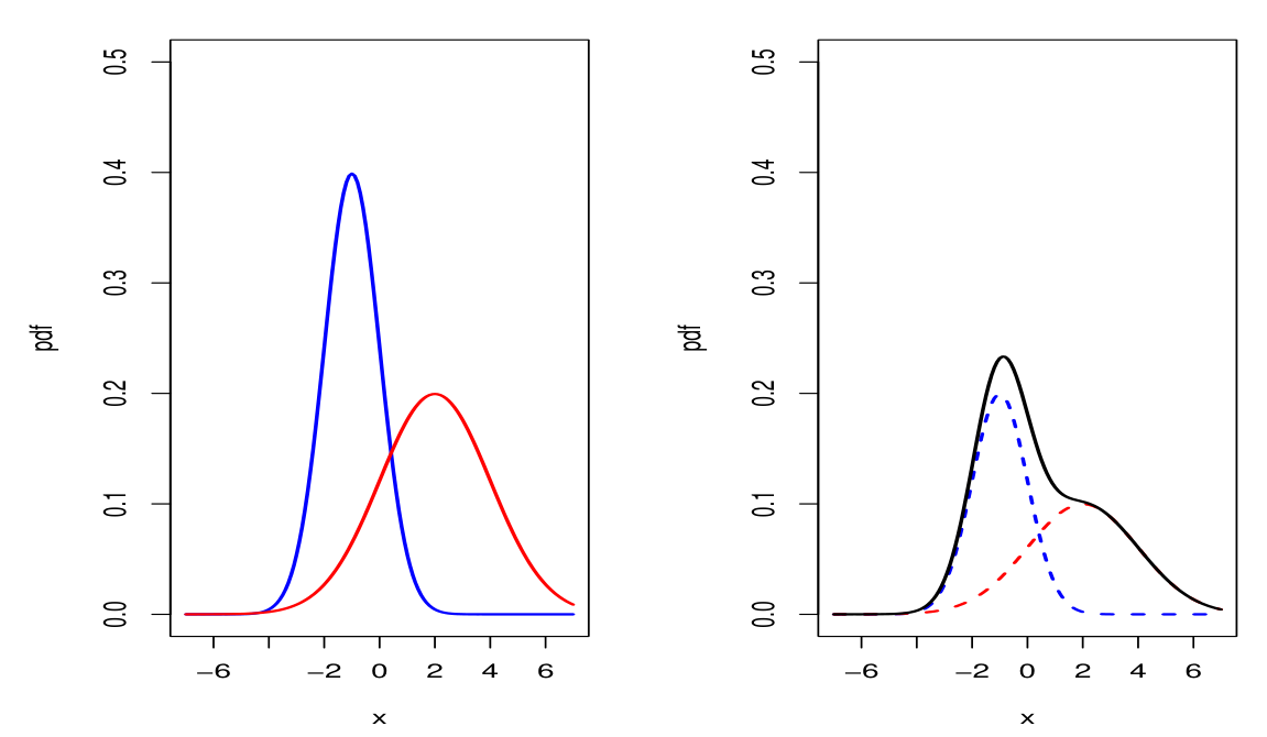
• Left plot
  • Blue line: $N(−1, 1^2)$
  • Red line: $N(2, 2^2)$
• Right plot
  • Blue dashed line: $0.5 \times N(−1, 1^2)$
  • Red dashed line: $0.5 \times N(2, 2^2)$
  • Black line: $0.5 \times N(−1, 1^2) + 0.5 \times N(2, 2^2)$

Sample Distribution

Distribution of Sample Mean

The sample mean $\bar{X}$ is a statistics representing the central tendency of samples.

• If the population mean is $\mu$, the sample mean serves as an estimator of $\mu$.

• For a random sample ${X_1, X_2, \cdots, X_n}$ drawn from a population with mean $\mu$ and variance $\sigma^2$, the sample mean is defined as:

  \[\bar{X} = \frac{1}{n} \sum_{i=1}^n X_i.\]

• For an infinite population:

  \[E(\bar{X}) = \mu, \, Var(\bar{X}) = \frac{\sigma^2}{n}, \, sd(\bar{X}) = \frac{\sigma}{\sqrt{n}}\]

• For a finite population of size $N$:

  \[E(\bar{X}) = \mu, \, Var(\bar{X}) = \frac{N - n}{N - 1} \cdot \frac{\sigma^2}{n}.\]

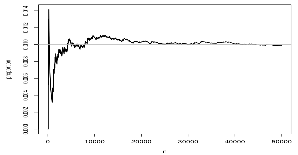
Law of Large Numbers (LLN)

The law of large numbers (LLN) states that as the sample size $n$ increases, the variance of the sample mean $\bar{X}$ approaches zero.

Since the expected value of the sample mean equals the population mean and the variance decreases as $n$ grows, $\bar{X}$ becomes increasingly concentrated around the population mean $\mu$. This phenomenon is what is referred to as the LLN.

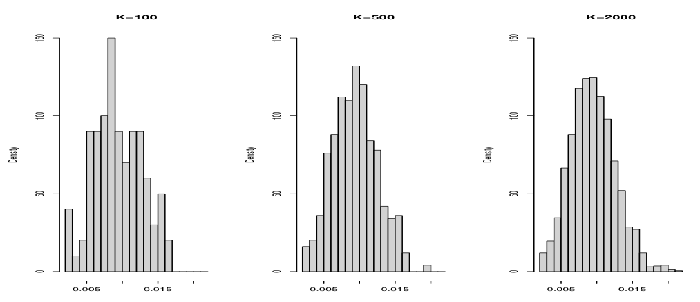
Central Limit Theorem (CLT)

The central limit theorem (CLT) states that for any population distribution, the distribution of

\[\frac{\bar{X} - \mu}{\sigma / \sqrt{n}}\]

approaches the standard normal distribution $N(0, 1)$ as $n$ becomes large.

In the case of a finite population, if the population size $N$ and sample size $n$ are sufficiently large (with $N \gg n$), the value of $\frac{N - n}{N - 1}$ approximates 1, allowing the property to hold.

The CLT implies that regardless of the shape of the population distribution, as the sample size increases, the distribution of the sample mean $\bar{X}$ can be approximated by a normal distribution.

• Specifically, the distribution of $\bar{X}$ is approximately:

  \[\bar{X} \sim N \left( \mu, \frac{\sigma^2}{n} \right).\]

Normal Approximation Using the Binomial Distribution

Let $X_1, X_2, \cdots, X_n$ be a random sample from a n infinite population following a Bernoulli distribution with success probability $p$. In this case, the sum $S = \sum_{i=1}^n X_i$ follows a binomial distribution $B(n, p)$.

By applying the CLT, for sufficiently large $n$:

\[\frac{S - np}{\sqrt{np(1 - p)}} = \frac{\hat{p} - p}{\sqrt{p(1 - p)/n}}\]

follows an approximate standard normal distribution $N(0, 1)$, where $\hat{p}=\frac{S}{n}$ is the sample proportion for the Bernoulli distribution.

Thus, if $n$ is sufficiently large and $np$ is a reasonable value, probability calculations involving $B(n, p)$ can be approximated using a normal distribution $N(np, np(1 - p))$.