Constrained Optimization

Constrained Optimization

General Constrained Optimization

\[\begin{aligned} & \text{minimize} & & f(x) \\ & \text{subject to} & & g_i(x) \le 0, \quad i=1,\dots,l\\ & & & h_j(x) = 0, \quad j=1,\dots,m\\ \end{aligned}\]

• $f$ : objective function.
• $g_i$ : inequality constraints.
• $h_j$ : equality constraints.
• The set of $x$ that satisfies the constraints is called the feasible set.
• $A(x)={i:g_i(x)=0} \cup {j:h_j(x)=0}$ is called the active set.
• For a given point \(x^*\) and the active set \(A(x^*)\), if \(\{\nabla g_i(x^*), i \in A(x^*)\}\) are linearly independent, then it is said that the LICQ (Linearly Independence Constraint Qualification) holds.

When the LICQ holds, the gradient of the active constraint cannot be 0.

• The problem can be rewritten as:

\[\begin{aligned} & \text{minimize} & & f(x) \\ & \text{subject to} & & \mathbf{g}(x) \le 0\\ & & & \mathbf{h}(x) = 0\\ \end{aligned}\]

• The Lagrangian of the problem is defined as follows:

\[L(x,\nu) = f(x) + \sum_{i=1}^l \lambda_i g_i(x) + \sum_{j=1}^m \nu_j h_j(x) = f(x) + \lambda^T \mathbf{g}(x) + \nu^T \mathbf{h}(x).\]

Karush-Kuhn-Tucker (KKT) Conditions

Motivation for the KKT Conditions

Consider an optimization problem with one inequality constraint.

\[\begin{aligned} & \text{minimize} & & f(x) \\ & \text{subject to} & & g(x) \le 0.\\ \end{aligned}\]

This can be expressed as follows:

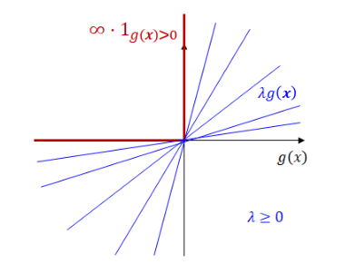
\[\begin{aligned} \text{minimize} \quad f_{\infty-step}(x) &:= \begin{cases} f(x) &\text{if } g(x)\le 0 \\ 0 &\text{if } g(x)> 0 \end{cases} \\ &= f(x) + \infty \cdot 1_{g(x)>0}. \end{aligned}\]

Here, $f_{\infty-step} = \max\limits_{\lambda \ge 0}$ $L(x,\lambda)$ where $L(x,\lambda)= f(x) + \lambda g(x)$.

Therefore, the optimization problem is newly expressed as follows:

\[\min\limits_{x}\max\limits_{\lambda \ge 0}L(x,\lambda) := f(x)+\lambda g(x).\]

KKT Conditions

Theorem: First-Order Necessary Conditions (KKT conditions)

Suppose that \(x^*\) is a local solution of constrained optimization problem and the LICQ holds at \(x^*\).

\[\begin{aligned} & \text{minimize} & & f(x) \\ & \text{subject to} & & g_i(x) \le 0, \quad i=1,\dots,l\\ & & & h_j(x) = 0, \quad j=1,\dots,m\\ \end{aligned}\]

Then there is a Lagrangian multiplier vector \((\lambda^*, \nu^*)\), such that the following KKT conditions are satisfied at \((x^*, \lambda^*, \nu^*)\):

\[\begin{aligned} &\text{(1)} \quad \nabla_x L(x^*,\lambda^*,\nu^*) = \nabla_x f(x^*) + \sum_{i=1}^l\lambda_i^*\nabla_x g_i(x^*) + \sum_{j=1}^m\nu_j^*\nabla_x h_j(x^*) = 0 \\ &\text{(2)} \quad g_i(x^*) \le 0, \forall i \\ &\text{(3)} \quad h_j(x^*) = 0, \forall j \\ &\text{(4)} \quad \lambda_i^* \ge 0, \forall i \\ &\text{(5)} \quad \lambda_i^* g_i(x^*) = 0, \forall i \end{aligned}\]

Each condition is called as follows:

• (1): Stationarity condition
• (2), (3): Primal feasibility condition
• (4): Dual feasibility condition
• (5): Complementary slackness condition

Lagrangian Duality

Primal and Dual Problem

• Primal problem

\[\begin{aligned} & \text{minimize} & & f(x) \\ & \text{subject to} & & g_i(x) \le 0, \quad i=1,\dots,l\\ & & & h_j(x) = 0, \quad j=1,\dots,m\\ \end{aligned}\]

or

\[\min\limits_{x}\max\limits_{\lambda \ge 0, \nu}L(x,\lambda,\nu) := f(x)+\lambda^T g(x)+\nu^T h(x)\]

• Lagrangian Dual problem

\[\max\limits_{\lambda \ge 0, \nu}D(\lambda,\nu):=\min\limits_{x}L(x,\lambda,\nu)\]

Duality Theorem

Weak Duality

The optimal value of the dual problem is a lower bound of the optimal value of the primal problem.

Theorem: Weak Duality

Let $x$ and $(\lambda,\nu)$ be a feasible solution to primal and dual problems, respectively. Then $f(x) \ge D(\lambda,\nu)$. Moreover, if \(f(x^*)=D(\lambda^*,\nu^*)\), then \(x^*\) and \((\lambda^*,\nu^*)\) solves the primal and dual problems, respectively.

• Duality gap: \(f(x^*)-D(\lambda^*,\nu^*)\)

Strong Duality

For a convex optimization problem, the optimal values of the dual problem and the primal problem are the same.

Theorem: Strong Duality

Let $f,g_i$ be convex and $h_j$ be affine for all $i,j$. Then \(f(x^*) = D(\lambda^*,\nu^*)\) if the optimal value is finite.

• Affine functions $f(x_1,…,x_n)=A_1x_1+…+A_nx_n+b$ 형태의 function.

Wolfe Duality

By using strong duality, a given optimization problem can be expressed in a different form.

Theorem: Wolfe Duality

Let $f,g_i$ be convex, $h_j$ be affine for all $i,j$, and \(x^*\) be an optimal solution of the primal. Then \((x^*,\lambda^*,\nu^*)\) at which LICQ holds solves the Wolfe dual problem of the form

\[\begin{aligned} & \text{minimize} & & L(x,\lambda,\nu) \\ & \text{subject to} & & \nabla_xL(x,\lambda,\nu)=0\\ & & & \lambda \ge 0\\ \end{aligned}\]

$\nabla_xL(x,\lambda,\nu)=0$ is the condition for $L(x,\lambda,\nu)$ to be the local optima.

Linear and Quadratic Programming

Linear Programming (LP)

\[\begin{aligned} & \text{minimize} & & c^Tx \\ & \text{subject to} & & Ax=b\\ & & & x \ge 0\\ \end{aligned}\]

• Lagrangian dual $L(x,\lambda,\nu) = c^Tx-\lambda^Tx+\nu^T(b-Ax)$ is convex.
• Therefore, the minimum is achieved when $c-\lambda-A^T\nu=0$ and $\lambda\ge 0$.
  • Check that $c-\lambda-A^T\nu=0$ and $\lambda\ge 0$ $\Longleftrightarrow$ $A^T\nu \le c$.
• As a result, the dual problem is given by:

\[\begin{aligned} & \text{maximize} & & b^T\nu \\ & \text{subject to} & & A^T\nu \le c.\\ \end{aligned}\]

Quadratic Programming (QP)

\[\begin{aligned} & \text{minimize} & & \frac{1}{2}x^THx+d^Tx \\ & \text{subject to} & & Ax \le b\\ \end{aligned}\]

where $H$ is symmetric and positive semidefinite. (Thus, the objective function is convex.)

• Lagrangian dual $L(x,\lambda) = \frac{1}{2}x^THx+d^Tx+\lambda^T(Ax-b)$ is convex.
• Therefore, the minimum is achieved when $Hx+A^T\lambda+d=0$ or $x=-H^{-1}(d+A^T\lambda)$.
• As a result, the dual problem is given by:

\[\begin{aligned} & \text{maximize} & & \frac{1}{2}\lambda^TD\lambda+\lambda^Tc-\frac{1}{2}d^TH^{-1}d \\ & \text{subject to} & & \lambda \ge 0\\ \end{aligned}\]

where $D=-AH^{-1}A$ and $c=-b-AH^{-1}d$.

This dual problem is simply a concave quadratic function maximization over a nonnegative domain, so it can be relatively easily solved.