Actor-Critic Policy Gradient
Actor-Critic Policy Gradient
Monte-Carlo policy gradient, 또는 REINFORCEMENT 알고리즘의 경우 variance가 무척 크다는 단점이 있다. 즉, 정밀한 estimation을 위해서는 아주 많은 computing이 필요하다. 이러한 이유로, action-value function $Q^{\pi_\theta}(s,a)$에 대한 더 나은 estimation을 찾기 위한 방법론들이 제안되었다.
그 중 하나로, critic을 이용하여 $Q^{\pi_\theta}(s,a)$를 예측하는 방법이 제안되었다. 이를 actor-critic algorithm이라고 한다.
\[Q_w(s,a) \approx Q^{\pi_\theta}(s,a)\]Actors and Critics
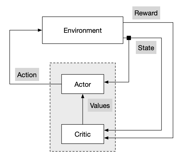
Actor-critic algorithm은 각각 parameter $w, \theta$를 갖는 두 종류의 함수 critic과 actor을 이용한다.
Critic은 parameter $w$를 갖는 action-value function $Q_w(s,a)$를 update하는 역할을 갖고, actor는 critic의 suggestion (계산 결과)를 기반으로 parameter $\theta$를 갖는 policy $\pi_\theta$를 update한다.
Critic은 현재 policy를 평가하는 역할, actor는 평가를 기반으로 현재 policy를 개선하는 역할이다. 따라서, 일종의 policy iteration으로 볼 수 있다.
Actor-critic algorithm은 $Q^{\pi_\theta}(s,a)$를 $Q_w(s,a)$로 추정하기 때문에, 아래 식을 이용하여 policy gradient를 진행한다.
\[\nabla_\theta J(\theta) \approx \ \mathbb{E}_{\pi_\theta} [\nabla_\theta \log \pi_\theta(s, a) Q_w(s,a)]\] \[\Delta \theta_t = \alpha \nabla_\theta \log \pi_\theta(s_t, a_t) Q_w(s,a)\]Action-Value Actor-Critic
Critic의 목표는 policy evaluation, 즉 $Q_w(s,a)$를 추정하는 것이다.
현실의 대부분의 문제는 state-action space가 무척 크기 때문에, $Q_w(s,a)$를 추정하기 위해서 neural network를 사용하지만, 여기서는 $Q_w(s,a)$가 linear function을 가지며 TD(0) 알고리즘을 통해 $w$를 업데이트한다고 가정하자.
이 경우, 간단한 actor-critic algorithm의 pseudocode는 다음과 같다.
- $Q_w(s,a) = \phi(s,a)^T w$
- Critic: TD(0) algorithm으로 update $w$
- Actor: policy gradient으로 update $\theta$
- 초기화: $s, \theta$
- Sampling: $a \sim \pi_\theta$
- 하기 과정(1 ~ 6)을 반복
- reward $r$와 next state $s’$ 얻음
- next action $a’ \sim \pi_\theta(s’, a’)$ 얻음
- $\delta = r + \gamma Q_w(s’,a’) - Q_w(s,a)$
- $\theta = \theta + \alpha \nabla_\theta \log \pi_\theta(s_t, a_t) Q_w(s,a)$
- $w = w + \beta\delta\phi(s,a)$
- $a \leftarrow a’, s \leftarrow s’$
Bias and Variance in Actor-Critic Algorithms
Actor-critic algorithm에서 가장 중요한 부분은 $Q_w(s,a)$를 어떤 함수로 선택할 것인지이다. $Q_w(s,a)$는 필연적으로 bias와 variance를 가지기 때문에, 적절하지 못한 함수를 선택하게되면 학습이 제대로 되지 않게된다.
Bias in Actor-Critic Algorithms
다행이도, bias는 문제가 되지않도록 만드는 방법이 알려져있다.
Theorem: Compatible Function Approximation
만약 하기 두 condition이 만족되는 경우,
Value function approximator is compatible to the policy
\[\nabla_w Q_w(s,a) = \nabla_\theta \log \pi_\theta(s,a)\]Value function parameters $w$ minimize the mean-squared error
\[\varepsilon = \mathbb{E}_{\pi_\theta} [(Q^{\pi_\theta}(s,a) - Q_w(s,a))^2]\]policy gradient 값을 다음 식을 통해 얻을 수 있다.
\[\nabla_\theta J(\theta) = \ \mathbb{E}_{\pi_\theta} [\nabla_\theta \log \pi_\theta(s, a) Q_w(s,a)]\]
Reducing Variance Using a Baseline
Variance를 줄이는 방법으로 baseline $B(s)$을 이용하는 방법이 있다. Baseline이란 state의 함수로, 다음 식이 성립한다.
\[\nabla_\theta J(\theta) = \ \mathbb{E}_{\pi_\theta} [\nabla_\theta \log \pi_\theta(s, a) Q^{\pi_\theta}(s,a)]\] \[\Rightarrow \nabla_\theta J(\theta) = \ \mathbb{E}_{\pi_\theta} [\nabla_\theta \log \pi_\theta(s, a) (Q^{\pi_\theta}(s,a)-B(s))]\]Baseline을 이용하면, expectation 값을 변경시키지 않고 variance를 줄일 수 있다.
\[\begin{aligned} \mathbb{E}_{\pi_\theta}\left[\nabla_\theta \log \pi_\theta(s, a) B(s)\right] &= \sum_s d^{\pi_\theta}(s) \sum_a \nabla_\theta \pi_\theta(s, a) B(s) \\ &= \sum_s d^{\pi_\theta}(s) B(s) \nabla_\theta \sum_a \pi_\theta(s, a) \\ &= \sum_s d^{\pi_\theta}(s) B(s) \nabla_\theta 1 = 0 \end{aligned}\]Advantage Function
Baseline function으로 state value function $V^{\pi_\theta}(s)$를 사용하면 좋은 성능을 보여준다. 이 때, advantage function $A^{\pi_\theta}(s,a)$을 다음과 같이 정의할 수 있다.
\[A^{\pi_\theta}(s,a) = Q^{\pi_\theta}(s,a) - V^{\pi_\theta}(s)\]Advantage function을 이용하면 policy gradient를 다음과 같이 쓸 수 있다.
\[\nabla_\theta J(\theta) = \ \mathbb{E}_{\pi_\theta} [\nabla_\theta \log \pi_\theta(s, a) A^{\pi_\theta}(s,a)]\]Advantage function은 variance reduction 측면에서 큰 장점을 가지고 있어 일반적으로 critic은 advantage function을 추정하게 된다.
Advantage function을 추정하기 위해서는 TD error $\delta^{\pi_\theta}$를 활용한다.
\[\delta^{\pi_\theta} = r + \gamma V^{\pi_\theta}(s') - V^{\pi_\theta}(s)\]TD error는 advantage function의 unbiased estimate이다.
\[\begin{aligned} \mathbb{E}_{\pi_\theta}\left[\delta^{\pi_\theta} \mid s, a\right] &= \mathbb{E}_{\pi_\theta}\left[r + \gamma V^{\pi_\theta}(s') \mid s, a\right] - V^{\pi_\theta}(s) \\ &= Q^{\pi_\theta}(s, a) - V^{\pi_\theta}(s) = A^{\pi_\theta}(s, a) \end{aligned}\]따라서, TD error를 이용하면 policy gradient를 다음과 같이 쓸 수 있다.
\[\nabla_\theta J(\theta) = \ \mathbb{E}_{\pi_\theta} [\nabla_\theta \log \pi_\theta(s, a) \; \delta^{\pi_\theta}]\]하지만, true value function 값을 미리 알 수는 없기 때문에, 다음과 같이 TD error에 대한 approximation을 사용한다.
\[\delta_v = r + \gamma V_v(s') - V_v(s)\]TD error를 추정하기 위해서는 value function에 대한 추정이 필요하다. 따라서, critic은 $Q^{\pi_\theta}(s,a)$와 $V^{\pi_\theta}(s)$를 동시에 추정한다.
\[Q_w(s,a) \approx Q^{\pi_\theta}(s,a), \quad V_v(s) \approx V^{\pi_\theta}(s)\] \[A(s,a) = Q_w(s,a) - V_v(s)\]
Critics at Different Time-Scale
Critic은 value function $V_v(s)$에 대한 추정을 다음과 같이 다양하게 진행할 수 있다.
MC: target은 return $G_t$가 된다.
\[\Delta v_t = \alpha(G_t - V_v(s))\phi(s)\]TD(0): target은 TD target $r + \gamma V(s’)$가 된다.
\[\Delta v_t = \alpha(r + \gamma V(s') - V_v(s))\phi(s)\]TD($\lambda$): target은 TD target $G_t^\lambda$가 된다.
\[\Delta v_t = \alpha(G_t^\lambda - V_v(s))\phi(s)\]
Actors at Different Time-Scale
Actor 역시 policy gradient에 대한 추정을 다양하게 진행할 수 있다.
\[\nabla_\theta J(\theta) = \mathbb{E}_{\pi_\theta} [\nabla_\theta \log \pi_\theta(s, a) A^{\pi_\theta}(s,a)]\]MC policy gradient: return $G_t$ 사용
\[\Delta \theta_t = \alpha(G_t - V_v(s_t))\nabla_\theta \log \pi_\theta(s_t, a_t)\]Actor-critic policy gradient: one-step TD error 사용
\[\Delta \theta_t = \alpha(r + \gamma V(s_{t+1}) - V_v(s_t))\nabla_\theta \log \pi_\theta(s_t, a_t)\]TD($\lambda$): TD target $G_t^\lambda$ 사용
\[\Delta \theta_t = \alpha(G_t^\lambda - V_v(s_t))\nabla_\theta \log \pi_\theta(s_t, a_t)\]
Summary of Policy Gradient
Policy gradient는 다음과 같이 다양한 형태를 가질 수 있다.
\[\begin{aligned} \nabla_\theta J(\theta) &= \mathbb{E}_{\pi_\theta}\left[\nabla_\theta \log \pi_\theta(s, a) \, G_t\right] \quad &\text{REINFORCE} \\ &= \mathbb{E}_{\pi_\theta}\left[\nabla_\theta \log \pi_\theta(s, a) \, Q_w(s, a)\right] \quad &\text{Q Actor-Critic} \\ &= \mathbb{E}_{\pi_\theta}\left[\nabla_\theta \log \pi_\theta(s, a) \, A(s, a)\right] \quad &\text{Advantage Actor-Critic} \\ &= \mathbb{E}_{\pi_\theta}\left[\nabla_\theta \log \pi_\theta(s, a) \, \delta\right] \quad &\text{TD Actor-Critic} \end{aligned}\]즉, policy gradient 알고리즘은 어떤 방법으로 policy gradient에 대한 estimation을 진행하느냐에 따라 다양한 방법이 존재한다.
하지만, policy gradient는 학습이 불안정하고, local optimum에 빠지기 쉬우며, sample을 효율적으로 사용하기 어렵다는 단점이 있어, 실질적으로 사용되기 어려웠다. 따라서, 이를 보완한 알고리즘들(TRPO, PPO 등)이 이후 다양하게 고안되었다.